Potu, Teja; Hu, Yunfei; Wang, Judy; Chi, Hongmei; Khan, Rituparna; Dharani, Srinija; Ni, Jingchao; Zhang, Liting; Zhou, Xin Maizie; & Mallory, Xian Fan. (2026). SCGclust: Single-cell graph clustering using graph autoencoders that integrate SNVs and CNAs. Mathematics, 14(1), 46. https://doi.org/10.3390/math14010046
Intra-tumor heterogeneity, or ITH, refers to the differences between cells within a single tumor, which can affect cancer outcomes and treatment responses. Single-cell DNA sequencing (scDNA-seq) allows researchers to study these differences at the level of individual cells. Low-coverage scDNA-seq can analyze many cells, but accurately grouping or clustering cells is essential to understand the tumor’s complexity. Most existing methods use either single-nucleotide variations (SNVs) or copy number alterations (CNAs) alone to cluster cells, even though both types of signals reflect subpopulations within the tumor. To address this, we developed a new cell-clustering tool that combines SNV and CNA information using a graph autoencoder. This model is trained alongside a graph convolutional network to ensure meaningful clusters and prevent all cells from being grouped together. The resulting low-dimensional cell representations are then clustered using a Gaussian mixture model. When tested on eight simulated datasets and one real cancer sample, our method outperformed existing SNV-only and CNA-only approaches, showing that integrating both types of genetic information improves the accuracy of identifying distinct cell populations within tumors.
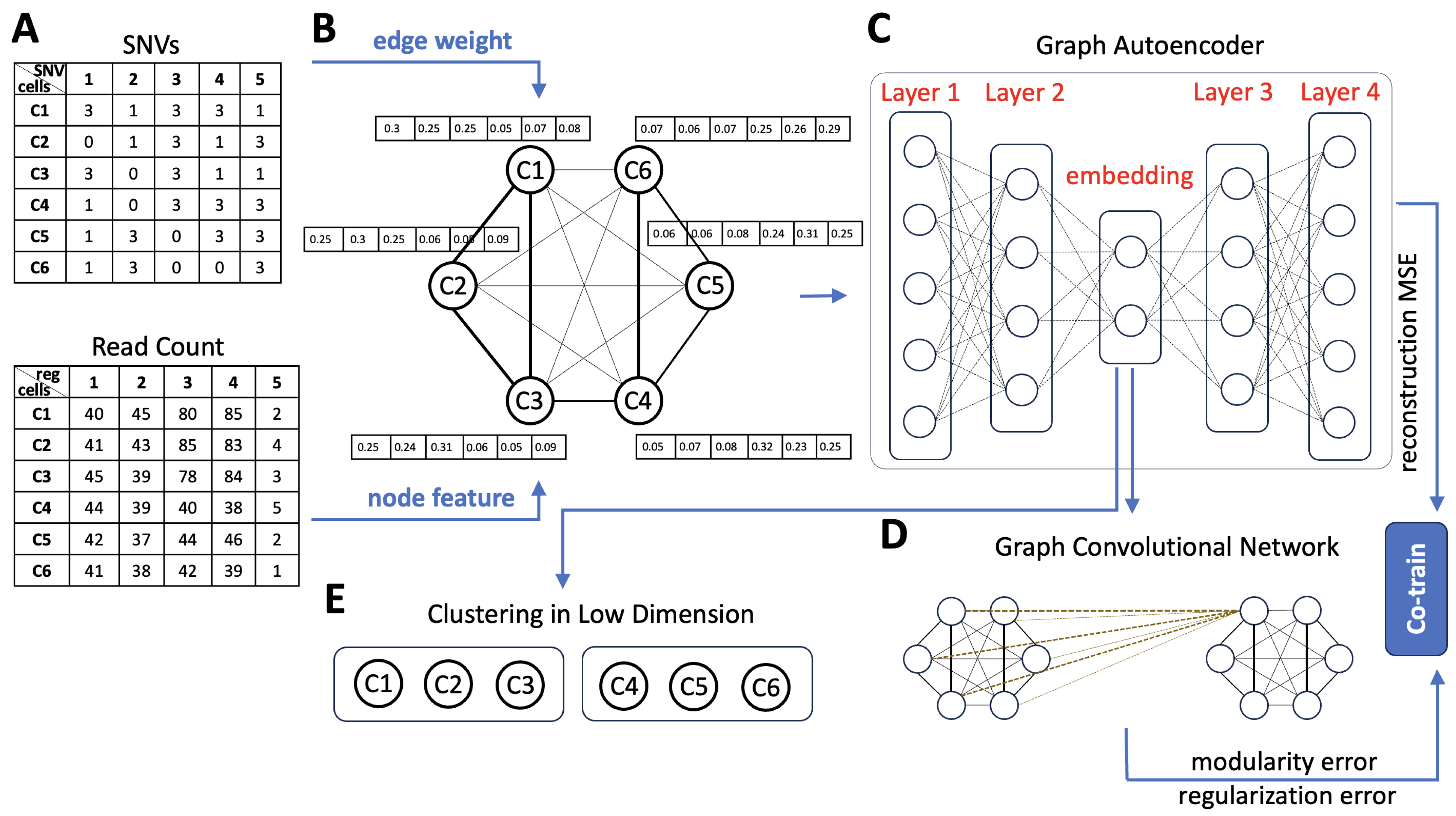
Figure 1. Overview of SCGclust. (A). There are two inputs to SCGclust, the cell by SNV matrix (top) and the cell by genomic region matrix (bottom). The cell by SNV matrix has entries “1”, “0”, and “3”. The “1” and “0” entries represent that the SNV is present or absent in the cell, respectively. The “3” entries represent that there is no read covering the site, and thus, the signal is missing. The cell by genomic region matrix has the read count for each genomic region at each cell. Six cells (C1–C6) are shown as an illustration. It can be observed that C1–C3 and C4–C6 have relatively similar SNV and CNA profiles, respectively. (B). The two matrices are then used as the edge weight and the node feature for the graph autoencoder. The graph autoencoder has six nodes, representing the six cells. On top of each node is a vector of the node feature, which uses the cosine similarity vector of the read count that reflects the CNA signal. Between every two nodes is an edge weight, represented by the Euclidean distance of the SNV profiles between the two cells. Here, C1, C2, and C3 have larger edge weights (thicker edges) because their SNV profiles are closer to each other. Similarly, C4, C5, and C6 have larger edge weights (thicker edges). (C). The built graph is the input for the graph autoencoder, which reduces the dimensions of the node features in the encoder and recovers the original node features in the decoder. The dimension reduction process also considers the edge weight such that two cells with similar SNV profiles will have more similar embedding in the low dimension. The graph autoencoder has four layers in total; layers 1 and 2 are the encoder, and layers 3 and 4 are the decoder. (D). A graph convolutional network (GCN) is co-trained with the graph autoencoder, with the objective function composed of three terms: the reconstruction mean squared error (MSE) term, the modularity term, and the collapse regularization term. (E). Finally, we performed the cell clustering based on each cell’s embedded low dimension from the graph autoencoder using the Gaussian mixture model.