Using R for Stylometric Analysis with the Stylo package

Stylometry is the analysis of linguistic style.  It is used primarily for authorial attribution.

You don’t actually need advanced computational statistics packages like R to conduct stylometric analysis, but they make the work much easier and enable analysis of extremely large text corpora.  Also: stylometry also offers a relatively intuitive way of understanding how statistical modeling can be useful for textual analysis.

Everyone reading this is likely familiar with the kind of basic text analysis that goes into generating word clouds, for example:

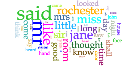
Word Cloud representing word frequency in Jane Eyre, created with Voyant tools https://cdn.vanderbilt.edu/vu-URL/wp-content/uploads/sites/214/2016/11/19221641/B2cXxjvV3EYBAAAAAElFTkSuQmCC.png

The kind of text mining we’re introducing today involves exploratory data analysis and predictive statistical modeling–not just counting words, but assessing the probability of correlation between datasets based on the likelihood that salient features will be shared between them.

Here: “dataset” = “novel”

And “salient features” = small, non-load-bearing words used most frequently.

It’s a core tenet of this kind of stylometric analysis that small, almost-unconsicously-used words can provide the best “signature” for an author’s style.

For example, in a 1964 study of the Federalist Papers, researchers found such differences in the writing styles of Alexander Hamilton and James Madison, such that, “only Madison used the word “whilst” (Hamilton used “while” instead). More subtly, while both Hamilton and Madison used the word “by,” Madison used it much more frequently, enough that you could guess who wrote which papers by looking at how frequently the word was used.”  (See Patrick Juola: https://www.scientificamerican.com/article/how-a-computer-program-helped-show-jk-rowling-write-a-cuckoos-calling/ .)

We can use Stylo to predict whether a new, unattributed, text will show the same features as a text known to be authored by a particular person.

The Stylo package in R pulls together a collection of specialized functions and commands to make this kind of analysis easier.  It includes a graphical user interface, to help make statistical stylometry accessible to neophytes, and it also comes pre-loaded with a few sample datasets that were assembled around contemporary questions of literary authorship and authorial attribution.

So let’s get started by loading up the Stylo package.

Launch R Studio

Create a new folder on your desktop. Call it “R_Workshop”

Create a new folder in R_Workshop folder.  Call it “corpus”

Let’s create a corpus for analysis later in this session.  Go to Project Gutenberg  https://www.gutenberg.org/ and select a few texts you would like to compare.  Note that you must use more than two texts.

Right-click on the plain text file link and “save link as”.  Use this format for file titles:  Authorname_textname.  Save files to the “corpus” sub-folder.

Now let’s download the Stylo script we’ll use for analysis.  Go to  https://sites.google.com/site/computationalstylistics/stylo/scripts and download (ver. 0.4.9.2).

Move the script into your R_Workshop folder.

Next, in R studio, type:

getwd()

This shows you what your current working directory is.  Change it to the new R_worskhop folder.

setwd(“C:/Users/PAUser/Desktop/R_Workshop”)

Now invoke the Stylo library and script:

library(stylo)

source(“stylo_0-4-9-2.r”)

This shows you Stylo’s graphical user interface, which we won’t work with just yet.  Let’s instead start out by looking at some of Stylo’s pre-loaded datasets.

data(galbraith)

rownames(galbraith)

Now type:

stylo(frequencies = galbraith, analysis.type = “CA”, write.png.file = TRUE, custom.graph.title = “Robert Galbraith”, gui = FALSE)

What you see here is a cluster analysis dendrogram, a visual representation of the statistical similarity of these texts in the dataset. If you’re curious, the math behind cluster analysis looks something like this:

Let the distance between clusters i and j be represented as dij and let cluster i contain ni objects. Let D represent the set of all remaining dij . Suppose there are N objects to cluster.

Find the smallest element dij remaining in D.

Merge clusters i and j into a single new cluster, k.

Calculate a new set of distances dkm using the following distance formula.

dkm = α idim +α jd jm + βdij + dim − d jm γ 8.00 6.00 4.00 2.00 0.00

Here m represents any cluster other than k. These new distances replace dim and d jm in D. Also let nk = ni + n j . Note that the eight algorithms available represent eight choices for α i ,α j , β, and γ .

Repeat steps 1 – 3 until D contains a single group made up of all objects. This will require N-1 iterations.

Now let’s test out another of Stylo’s existing datasets.

data(lee)

rownames(lee)

Type:

stylo(frequencies = lee, analysis.type = “CA”, write.png.file = TRUE, custom.graph.title = “Harper Lee”, gui = FALSE)

Now type:

stylo(frequencies = lee, analysis.type = “CA”, mfw.min = 1500, mfw.max = 1500, custom.graph.title = “Harper Lee”, write.png.file = TRUE, gui = FALSE)

Take a close look at the two graphs and the scripts that produced them.  What are the differences?

Finally, let’s launch the graphical user interface and run a quick analysis on some texts of your choice.  What are your findings?

https://www.scientificamerican.com/article/how-a-computer-program-helped-show-jk-rowling-write-a-cuckoos-calling/