Sensitivity to initial conditions
Another important feature emerges in the chaotic region ...
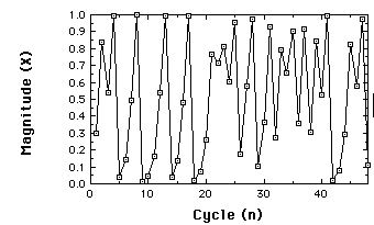
To see it, we set r=3.99 and begin at x1=.3. The next graph shows the time series for 48 iterations of the logistic map.
 Time series for Logistic map r=3.99, x1=.3, 48
iterations.
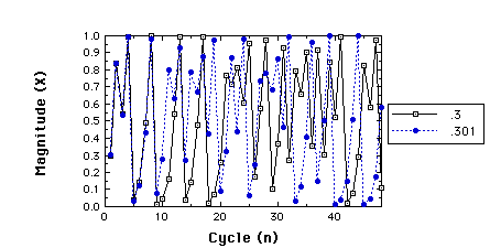
Now, suppose we alter the starting point a bit. The next figure compares the time series for x1=.3 (in black) with that for x1=.301 (in blue).
 Two time series for r=3.99, x1=.3 compared to
x1=.301
The two time series stay close together for about 10 iterations. But after that, they are pretty much on their own.
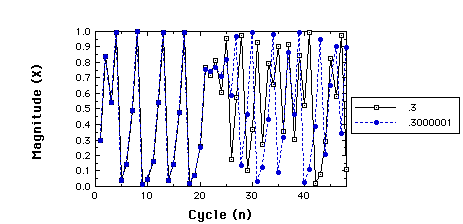
Let's try starting closer together. We next compare starting at .3 with starting at .3000001...
 Two time series for r=3.99, x1=.3 compared to
x1=.3000001
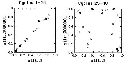
This time they stay close for a longer time, but after 24 iterations they diverge. To see just how independent they become, the next figure provides scatterplots for the two series before and after 24 iterations.
 Scatterplots of series starting at .3 vs. series starting at
.3000001.
The
first 24 cycles on the left, next 24 on the right.
The correlation after 24 iterations (right side), is essentially zero. Unreliability has replaced reliability.
We have illustrated here one of the symptoms of chaos. A chaotic system is one for which the distance between two trajectories from nearby points in its state space diverge over time. The magnitude of the divergence increases exponentially in a chaotic system.
So what? Well, it means that a chaotic system, even one determined by a simple rule, is in principle unpredictable. Say what? It is unpredictable, "in principle" because in order to predict its behavior into the future we must know its currrent value precisely. We have here an example where a slight difference, in the sixth decimal place, resulted in prediction failure after 24 iterations. And six decimal places far exceeds the kind of measuring accuracy we typically achieve with natural biological systems.
Next Section: Symptoms of Chaos