Paper presented at MPA, Chicago, May, 1995

     Here is the central thesis of this paper. If time series data are 
the result of a nonlinear dynamic system, then techniques are available for 
estimating the number of dynamic variables that produced the data. We 
recommend an experimental paradigm in which the independent variables 
are those known to influence performance, and the dependent variables are 
estimates of dimensionality. This paradigm allows us to investigate 
whether the independent variable is influencing a dynamic variable, one 
that changes in time, or is affecting a relatively constant system parameter. 
We apply this paradigm to some memory data here, but we offer it as a 
general experimental paradigm. That's the message. The rest of this paper 
is devoted to details of definition, illustration, and a brief discussion of 
limitations.

     What do we mean by a dynamic model? A dynamic model is any 
model for which some measure x changes over time according to 
an explicit function. A nonlinear dynamic model is simply one for which the 
equation specifying the change is not linear. The simplest example of a 
discrete nonlinear model is the logistic map, for which x changes 
from time n to time n+1 according to:

     The logistic map is often used to introduce chaos concepts because, for 
certain values of the parameter r, the resulting dynamics display 
all the features of a chaotic system. It is important to stress that nonlinearity 
refers not to the behavior of x over n, but to the relation of x_n and x_(n+1).

     An unattractive feature of nonlinear models is their resistance 
to solution by formal analysis. On the other hand, recent work has yielded 
a number of geometric regularities and useful techniques for characterizing 
these systems and for discriminating them from other systems.

     A compelling feature of nonlinear systems is that even simple systems, 
such as the logistic map, produce behavior that is difficult to distinguish 
from random behavior. This is illustrated in the Figure 1, which shows a 
time series produced when r equals 4 and compares it with truly random 
data.

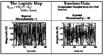Figure 1 Behavior of the Logistic map and Random Data.
     We take this apparently random behavior as a potential challenge to the 
conventional view of variability. The conventional view is that measures 
are the linear sum of true scores plus noisy "error", which in turn is the 
result of the contribution of a very large number of independent factors. 
The new insight is that seemingly random variability in measures over 
time can result from very simple deterministic systems.

     We use the term dynamic variable to refer to variables that change over 
time, to be distinguished from parameters which do not. In the logistic map 
example, x is a dynamic variable and r is a parameter. More generally, a 
dynamic system is a set of functions representing  N inputs and N outputs. 
For example, a discrete system would be represented by a set of N difference 
equations:

where x_i are dynamic variables and parameters are indexed by p_i. More 
simply: dynamic variables are indexed by time, parameters are not. There 
are N variables and K parameters. Notice that the dynamic variables are 
"coupled", which means that change in one depends on the current value 
of the other.

     The number of dynamic variables of a system is known as the 
dimensionality of the system. The logistic map, for example, has 
dimensionality equal to one.  An example of a two-dimensional dynamic 
system (Clayton & Frey, in press) is shown next.

     This model, similar to one suggested by van Geert (1991), has two 
dynamic variables, x and y, competing for growth according to growth 
parameters r_x and r_y but limited in magnitude by carrying capacity K. 
Here there are two dynamic variables and four parameters. The model also 
illustrates why we think that memory performance may be profitably 
modeled by a nonlinear system. Memory typically involves competition, 
and is limited in capacity, at least in working memory. The result is that the 
dynamic variables are "coupled" and growth is bounded. In addition to the 
van Geert work already cited, in recent years dynamic models have been 
proposed across psychology. See the reference list for a partial listing of this 
new work.

     One of the remarkable recent achievements in the study of nonlinear 
dynamics is the development of techniques for estimating dimensionality 
from measures on a single variable. Such techniques could be enormously 
useful to the model builder because they estimate the total number of 
dynamic variables needed to model the dependent variable.

     How is this possible? The major technique involves the embedding 
dimension, which is defined in terms of successive N-tuples of the time 
series data. Consider, for example, the first seven values of the logistic map 
data plotted earlier.  
0.10, 0.36, 0.92, 0.30, 0.84, 0.54, 0.99. ...
     For an embedding dimension of two, the resulting pairs are
(0.10, 0.36), (0.36, 0.92), (0.92, 0.30), (0.30, 0.84), (0.84, 0.54), (0.54, 0.99), ...

     For an embedding dimension of three, the triplets are
(0.10, 0.36, 0.92), (0.36, 0.92, 0.30), (0.92, 0.30, 0.84), (0.30, 0.84, 0.54), ...

     These successive N-tuples are treated as vectors, or points, in N-
dimensional space, and it is the geometric structure of these points that is of 
interest. To illustrate their utility, suppose we embed the time series from 
the logistic map in two dimensions and plot the points in 2-space. Figure 2 
shows the result. We see that the underlying structure of a system 
producing seemingly random data is fully revealed by embedding the data 
in two dimensions.

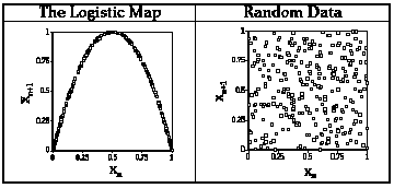
Figure 2. Return map drawn for the first 300 trials
of the Logistic map, r=4, and random data.

     Techniques for estimating dimensionality, in general, involve distances 
among the points in the embedding dimensions. And the central idea is 
that certain properties of these distances will change as the embedding 
dimension increases, but only so long as the embedding dimension is less 
than the dimensionality of the data.  In the particular technique developed 
by Grassberger and Procaccio (1983a,b), which rapidly became widely used in 
other sciences, for each embedding dimension the proportion of distances 
that are less than a given distance, or radius, r are calculated. This value is 
called the correlation integral, Cr(I), and the linear portion of the function 
relating log[Cr(I)] to log(r) is used to estimate the correlation dimension for 
that embedding dimension. 

     The next figure illustrates the technique applied to data from the logistic 
map and from data generated as white noise. 

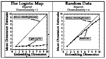
Figure 3. Estimates of correlation dimension as a
function of embedding dimension for
logistic map and white noise data.

     Plotted here are dimension estimates as a function of embedding 
dimension. The logic is this. As long as dimensionality exceeds the 
embedding dimension, the estimate will equal the embedding dimension. 
Since white noise has infinite dimensionality, estimates should 
continuously equal the embedding dimension, as they are seen to do. The 
logistic map data, however, are the result of a one-dimensional system and 
should not rise beyond an embedding of one. In general, then, we look to 
see whether and where this function levels off, or "saturates" as reaching an 
asymptote is called.

     Now, we argue, the ability to estimate the dimensionality of data 
arising from a given experimental condition invites a new paradigm in 
which the relationship between independent variables and dimensionality 
are investigated. The initial logic is this: if the independent variable 
influences both the dependent variable and the dimensionality estimate, its 
influence arises from its effect on a dynamic variable. If, however, the 
independent variable influences the dependent variable but not 
dimensionality, then its effect is on a parameter. The possible results are 
summarized in the next table.

     One limitation of this approach may already be apparent. If the estimate of 
dimensionality is very large, or too large to estimate, the suitability of the 
nonlinear approach would be questioned and the location of the effect of the 
independent variable it would be unclear. 

     We illustrate all of this with the experiment now to be described.

Experiment

     Three classification tasks were used, designed to manipulate memory load, 
so our major experimental question was whether memory load affects a 
dynamic variable or a parameter.

Method

     Twelve subjects were each given three classification tasks that differed only 
in the response rule. On each trial of each task the stimulus was either an X or 
an O.  In the X-O task, the subject pressed one key for an X, another for an O. 
In the same-different-1 task the subject pressed one key if the stimulus was 
the same as the stimulus on the previous trial, otherwise the other key. On 
the same-different-2 task, the subject pressed one key if the stimulus was the 
same as the stimulus two trials back, otherwise the other key. Each task had 
500 uninterrupted trials, with task order counterbalanced across subjects. We 
used 500 trials because the planned nonlinear statistics require lengthy time 
series.

     Reaction time was measured on each trial. In addition, since the subject 
determined the intertrial interval by indicating readiness for the next 
trial, it occurred to us  that the interesting temporal dynamics may be in this 
subject-determined delay. The subjects were encouraged to develop a strategy 
to prepare for the next trial, and this interval, too, was measured.

Results 

     The next figures display the obtained data using the standard plot of 
dependent variables vs. independent variables, and show the expected effect 
for both. Both response times and trial-initiation times increased significantly 
with increased memory load, being fastest for the simple X-O task, slowest for 
the task requiring memory for the last two trials.

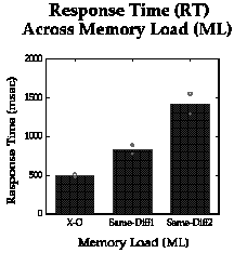
Figure 4a. Mean latencies (msec) for response
time across increasing memory load.


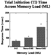
Figure 4b. Mean latencies (msec) for trial
initiation across increasing memory load.

     That's the standard analysis. Now we treat the data as a time series and 
examine  the effect of memory load on our new measure, dimensionality. 
Analyses of variance on Grassberger-Procaccia estimates showed no effect of 
memory load. That is, there was no evidence that memory load was affecting 
a dynamic variable, despite its substantial effect on response times. There was, 
however, also no evidence for low-dimensionality in the response time data. 
This is shown in the next figure.

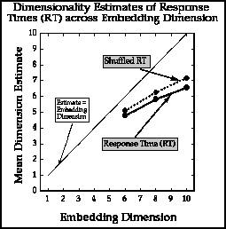
Figure 5. Slope estimates across embedding
dimensions for response times to test
stimulus, shuffled vs. non-shuffled data.

     This figure shows estimates from the response time data on the left, 
trial-initiation time on the right. Two functions of slope estimates across 
embedding dimensions are shown. The solid function is for the obtained 
data, the dashed line for the same data randomly shuffled. Shuffled data 
should resemble white noise, so shuffling controls against biased estimations. 
The technique is similar to the "surrogate data" method. (Theiler, Eubank, 
Longtin, Galdrikian, & Farmer, 1992; Theiler, Galdrikian, Longtin, Eubank, & 
Farmer,1992; Kennel  & Isabelle, 1993). The response time data show no 
evidence of saturating and no difference from the shuffled version. 

     The story is somewhat different for the trial initiation data shown in 
the next figure. 

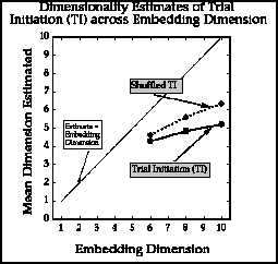
Figure 6. Slope estimates across embedding
dimensions for trial initiation times,
shuffled vs. non-shuffled data.

     Here there is a significant difference between the obtained and shuffled 
data. There is also a  suggestion that dimensionality estimates of the 
obtained data levels off, perhaps at a dimensionality of six.  Our maximum 
embedding dimension is ten here because the reliability of dimension 
estimates decrease as embedding dimension increases, especially for short 
data sets. So, without using other dimension estimates, which are planned, 
we tentatively conclude that low-dimensionality in the time-initiation data is 
possible.

     In summary, the memory load manipulation produced substantial 
effects on response and trial initiation times, but no effects on estimates of 
dimensionality.  We have used these data to illustrate the potential for an 
experimental paradigm that treats dimensionality as a dependenet variable. 
Provided dimensionality estimates are low, this technique provides evidence 
about whether the independent variable influences a dynamic varaible or a 
system parameter.

     Finally, nonlinear statistical techniques are very much in the 
developmental stage Several approaches have been suggested, and recent 
reviews of the strengths and weaknesses of the techniques are to be found in 
Abarbanel, Brown, Sidorowich, and Tsimring (1993), Pritchard and Duke 
(1992), Johnson and Dooley (1994), and Rapp (1995).
 

Abarbanel, H. D. I., Brown, R., Sidorowich, J. J. & Tsimring, L. S. (1993). 
     The analysis of observed chaotic data in physical systems. Reviews 
     of Modern Physics, 65, 1331-1392. 

Clayton, K. & Frey, B. (In press). Inter- and intra-trial dynamics in memory 
     and choice. In J. Goldstein & A. Coombs (Eds.), Chaos Psychology: A 
     Reader. Vol 2.

Cooney, J. B. & Troyer, R. (1994).  A dynamic model of reaction time in a 
     short-term memory task. Journal of Experimental Child 
     Psychology, 58, 200-226.

Grassberger, P., & Procaccia, I. (1983a). Characterization of strange 
     attractors. Physical Review Letters, 50, 346-349. 

Grassberger, P., & Procaccia, I. (1983b). Measuring the strangeness of 
     strange attractors, Physica D, 9, 189-208. 

Hoyert, M. S. (1992). Order and chaos in fixed-interval schedules of 
     reinforcement. Journal of the Experimental Analysis of Behavior, 
     57, 339-363. 

Pritchard, W. S. & Duke, D. W. (1992). Measuring chaos in the brain: A 
     tutorial review of nonlinear dynamical EEG analysis. International 
     Journal of Neuroscience, 67, 31-80. 

Townsend, J. T. (1992b). Chaos theory: A brief tutorial and discussion. 
     Ch. 4 in A. F. Healy, S. M. Kosslyn, & R. M. Shiffrin (Eds.) From 
     Learning Theory to Connectionist Theory: Essays in Honor of William 
     K. Estes, V.1. Hillsdale NJ: L. Erlbaum Assoc. pp.65-96.

van Geert, P. (1991). A dynamic systems model of cognitive and language 
     growth. Psychological Review, 98, 3-53.