SCTPLS Basic Workshop
 Basic Concepts in Nonlinear Dynamics
and Chaos
These pages are taken from a Workshop presented at the annual meeting of the Society for Chaos Theory in
Psychology and the Life Sciences
June 28,1996 at Berkeley, California.
© Keith Clayton
Other Web sites that treat introductory nonlinear dynamics and fractals are:
What is a dynamic system?
A dynamic system is a set of functions (rules, equations) specifying how variables change over time.
For example ...
Alice's height diminishes by half every minute...
Another example ...
x(new) = x(old) + y(old)
y(new)= x(old)
This last rule illustrates a system with two variables. Variable X is changed by taking its old value and adding the value of Y. And Y is changed by becoming X's old value. Silly system? Perhaps. We're just showing that a dynamic system is any well-specified set of rules.
Here are some important Distinctions:
- variables (dimensions) vs. parameters
- discrete vs. continuous variables
- stochastic vs. deterministic dynamic systems
How they differ:
- Variables change in time, parameters do not.
- Discrete variables are restricted to integer values, continuous
variable are not.
- Stochastic systems are one-to-many; deterministic
systems are one-to-one
This last distinction will be made clearer as we go along ...
Terms
The current state of a dynamic system is specified by the current value of its variables, x, y, z, ...
The process of calculating the new state of a discrete system is called iteration.
To evaluate how a system behaves, we need the functions, parameter
values and initial conditions or starting state.
To illustrate...Consider a classic learning theory, the alpha model, which specifies how q(n), the probability of making an error on trial n, changed from one trial to the next
q(n+1) = ß q(n)
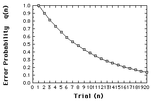
The new error probability is diminished by ß (which is less than 1, greater than 0). For example, let the the probability of an error on trial 1 equal to 1, and ß equal .9. Now we can calculate the dynamics by iterating the function, and plot the results.
q(1) = 1
q(2) = ßq(1) = (.9)(1) = .9
q(3) = (.9)q(2) = (.9)(.9) = .81
etc. ...
Error probabilities for the
alpha model, assuming q(1)=1, ß =.9.
This "learning curve" is referred to as a time series.
So far, we have some new ideas, but much is old ...
What's not new
Dynamic Systems
Certainly the idea that systems change in time is not new. Nor is the idea that the changes are probabilistic.
What's new
Deterministic nonlinear dynamic systems.
As we will see, these systems give us:
- A new meaning to the term unpredictable
- A different attitude toward the concept of variability
- Some new tools for exploring time series data and for modeling such behavior.
- And, some argue, a new paradigm.
This last point is not pursued here.
Back to Table of Contents
Nonlinear functions
What's a linear function?
Well, gee Mikey, it's one that can be written in the form of a straight line. Remember the formula? ...
y = mx + b
where m is the slope and b is the y-intercept?
What's a nonlinear function?
Any function that ain't linear!
Is the Alpha model a linear model?
Yes, because q(n+1) is a linear function of q(n)
But wait! Its output, the plot of its behavior over time (Figure 1 above) is not a straight line.Doesn't that make it a nonlinear system?
No, what makes a dynamic system nonlinear ....
is whether the function specifying the change is nonlinear.
Not whether its behavior is nonlinear.
And y is a nonlinear function of x if x is multiplied by another (non-constant) variable or by itself (that is, raised to some power).
We illustrate nonlinear systems using ...
Logistic Difference Equation
... a model often used to introduce chaos. The Logistic Difference Equation, or Logistic Map, though simple, displays the major chaotic concepts.
Growth model
We start, generally, with a model of growth.
x(new) = r x(old)
We prefer to write this in terms of n:
x(n+1) = r x(n).
This says x changes from one time period, n, to the next, n+1, according to r. If r is larger than one, x gets larger with successive iterations If r is less than one, x diminishes. (In the "Alice" example at the beginning, r is .5).
Let's set r to be larger than one...
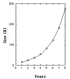
We start, year 1 (n=1), with a population of 16 [x(1)=16], and since r=1.5, each year x is increased by 50%. So years 2, 3, 4, 5, ... have magnitudes 24, 36, 54, ...
Our population is growing exponentially. By year 25 we have over a quarter million.
Iterations of Growth model with r = 1.5
So far, notice, we have a linear model that produces unlimited growth.
Limited Growth model - Logistic Map.
The Logistic Map prevents unlimited growth by inhibiting growth whenever it achieves a high level. This is achieved with an additional term, [1 - x(n)].
The growth measure (x) is also rescaled so that the maximum value x can achieve is transformed to 1. (So if the maximum size is 25 million, say, x is expressed as a proportion of that maximum.)
Our new model is
x(n+1) = r x(n) [1 - x(n)]
[r between 0 and 4.]
The [1-x(n)] term serves to inhibit growth because as x approaches 1, [1-x(n)] approaches 0.
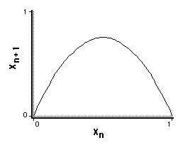
Plotting x(n+1) vs. x(n), we see we have a nonlinear relation.
Limited growth (Verhulst) model. X(n+1) vs. x(n), r =
3.
We have to iterate this function to see how it will behave ...
Suppose r=3, and x(1)=.1
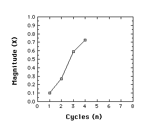
x(2) = r x(1)[1-x(1)] =
3(.1)(.9) =
.27
x(3 )= r
x(2)[1-x(2)]= 3(.27)(.73) = .591
x(4 )= r x(3)[1-x(3)]= 3(.591)(.409) =
.725
Behavior of the Logistic map for r = 3, x(1) = .1, iterated to give
x(2), x(3), and x(4)
It turns out that the logistic map is a very different animal, depending on its control parameter r. To see this, we next examine the time series produced at different values of r, starting near 0 and ending at r=4. Along the way we see very different results, revealing and introducing major features of a chaotic system.
When r is less than 1
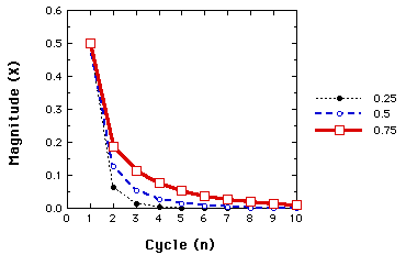 Behavior of the Logistic map for r=.25, .50, and .75. In all cases
x(1)=.5. The same fates awaits any starting value. So long as r is less than 1, x goes toward 0. This illustrates a one-point attractor.
When r is between 1 and 3
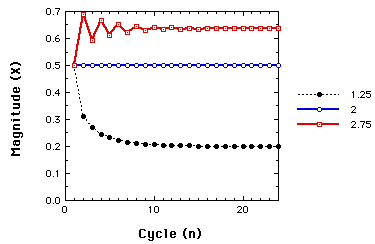 Behavior of the Logistic map for r=1.25, 2.00, and 2.75. In all
cases x(1)=.5.
Now, regardless, of the starting value, we have non-zero one-point attractors.
When r is larger than 3
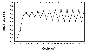 Behavior of the Logistic map for r=3.2.
Moving just beyond r=3, the system settles down to alternating between two points. We have a two-point attractor.
We have illustrated a bifurcation, or period doubling,
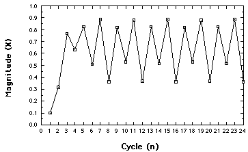 Behavior of the Logistic map for r= 3.54. Four-point
attractor
Another bifurcation. The concept: an N-point attractor.
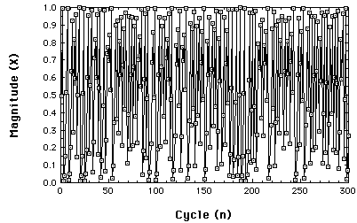 Chaotic behavior of the Logistic map at r=
3.99.
So, what is an attractor? Whatever the system "settles down
to".
Here is a very important concept from nonlinear dynamics: A system eventually "settles down". But what it settles down to, its attractor, need not have 'stability'; it can be very 'strange'.
Back to the Table of Contents
So, again, what is a bifurcation? A bifucation is a period-doubling, a change from an N-point attractor to a 2N-point attractor, which occurs when the control parameter is changed.
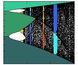
A Bifurcation Diagram is a visual summary of the succession of period-doubling produced as r increases. The next figure shows the bifurcation diagram of the logistic map, r along the x-axis. For each value of r the system is first allowed to settle down and then the successive values of x are plotted for a few hundred iterations.
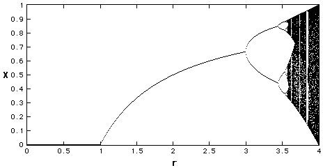 Bifurcation Diagram r between 0 and 4
We see that for r less than one, all the points are plotted at zero. Zero is the one point attractor for r less than one. For r between 1 and 3, we still have one-point attractors, but the 'attracted' value of x increases as r increases, at least to r=3. Bifurcations occur at r=3, r=3.45, 3.54, 3.564, 3.569 (approximately), etc., until just beyond 3.57, where the system is chaotic.
However, the system is not chaotic for all values of r greater than 3.57.
Let's zoom in a bit.
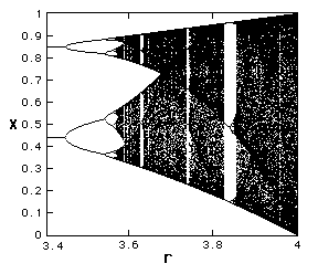 Bifurcation Diagram r between 3.4 and 4
Notice that at several values of r, greater than 3.57, a small number of x=values are visited. These regions produce the 'white space' in the diagram. Look closely at r=3.83 and you will see a three-point attractor.
In fact, between 3.57 and 4 there is a rich interleaving of chaos and order. A small change in r can make a stable system chaotic, and vice versa.
Back to Table of Contents
Another important feature emerges in the chaotic region ...
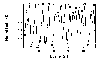 Time series for Logistic map r=3.99, x(1)=.3, 48
iterations.
Suppose I have two near-by starting points.
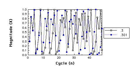 Two time series for r=3.99, x(1)=.3 compared to
x(1)=.301
Perhaps I didn't start close together enough ...
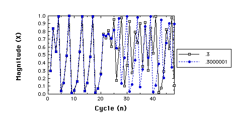 Two time series for r=3.99, x(1)=.3 compared to
x(1)=.3000001
Check the correlation before and after they diverge ...
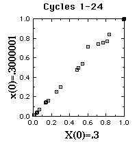
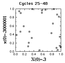 Scatterplots of series starting at .3 vs. series starting at
.3000001.
The
first 24 cycles on the left, next 24 on the right.
Back to the Table of Contents
- apparent randomness
- deterministic
- sensitive to 'initial' conditions
Important restriction: None of these alone are sufficient
conditions.
Note on technical vs. metaphorical uses of terms:
- 'bifurcation' - technically, not a dynamic change
- 'chaos' - technically, not 'overwhelming anxiety'
Back to the Table of Contents
We practice the distinction between variables (dimensions) and
parameters
Consider again the Logistic map
x(n+1) = r x(n)[1- x(n)]
Multiply the right side out
x(n+1)= r x(n) - r x(n)^2,
and replace the two r's with separate parameters, a and b,
x(n+1)= a x(n) - b x(n)^2,
Separate parameters now govern growth and suppression, a and b, but we
still have only one variable, x.
When we have a system with two or more dimensions,
- its current state is the current values of its variables, and
- treated as a point in phase (state) space, and
- we refer to its trajectory or orbit in time.
Predator-prey system
A two-dimensional dynamic system in which two variables grow, but one
grows at the expense of the other.
The number of predators is represented by y, the number of prey by x.
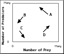
A = Too many
predators
B = Too few prey
C = Few predator and
prey. Prey can grow
D= Few predators, ample prey
�
The phase-space of the predator-prey system.
The resulting trajectory (idealized)...
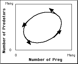 The phase-space of the predator-prey system.
An attractor that forms a loop like this is called a limit cycle.
If the system starts from other points ...
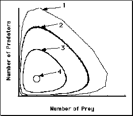 Phase-portrait of the predator-prey system, showing the
influence of starting state.
Points 1-4 start with about the same number of prey but with different
numbers of predators.
Let's look at this system as a time series.
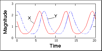 The time series of the predator-prey system.
Showing the oscillations, out of phase, of the magnitudes of the predator
and prey populations.
Continuous Functions and Differential Equations
- Changes in discrete variables are expressed with difference
equations, such as the logistic map.
- Changes in continuous variables are expressed with differential
equations
For example, the Predator-prey system is typically presented as a set of
two differential equations:
dx/dt = (a-by)x
dy/dt = (cx-d)y
Another two-dimensional continuous dynamic system...
The Buckling column system
Used by Abraham, Abraham, & Shaw (1990) as a starting point to discuss
psychological phenomena that exhibit oscillations (for example, mood
swings, states of consciousness, attitude changes).
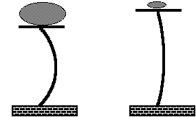 The buckling column model. Reproduced from Abraham,
Abraham, & Shaw (1990).
On the left, the mass is sufficient to cause the vertical column to buckle.
x represents sideways displacement of the middle of the
column.
y stands for the velocity of its movement.
dx/dt = y
dy/dt = (1 - m)(ax^3 + b + cy)
With a light mass (m) and friction (c), the column eventually returns to the
upright position:
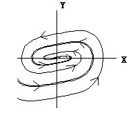 Phase portrait of the buckling column model.
With a heavy mass, the column comes to rest in one of two positions (two-
point attractor).
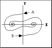 Phase portrait of the buckling column model.
Basins of attraction
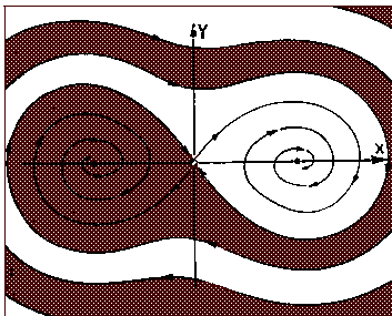 The basins of attraction for the buckling column system.
Reproduced from Abraham et al (1990).
The term seperatrix is used to refer to the boundary between
basins of attraction.
Types of two-dimensional interactions - van Geert (1991)
- mutually supportive - the larger one gets, the faster the other grows
- mutually competitive - each negatively affects the other
- supportive-competitive - as in Predator-prey
Three-dimensional Dynamic Systems
The Lorenz System
A now classic model of atmospheric dynamics
dx/dt = a(y-x)
dy/dt = x(b-z) - y
dz/dt = xy-cz
The first strange attractor, the icon for chaos.
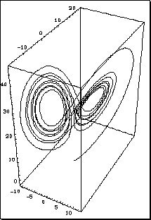 The Lorenz system. Only a portion of a trajectory is shown.
Beasts in Phase space - Limit Points
- Attractors - where the system 'settles down' to.
- Repellors - a point the system moves away from.
- Saddle points - attractor from some regions, repellor to others.
Examples
- Attractors - we've seen many
- Repellors - the value 0 in the Logistic Map
- Saddle points - the point (0,0) in the Buckling Column
Nonlinear Dynamics, Psychology & Life Sciences (Resumed
again)
1. Phenomena may be measured in one dimension, but "determining"
variables comprise other dimensions in a dynamic phase space.
2. The measures not the sum of the effects of a set of independent
variables( each unaffected by the value of the dependent measure), plus
random error.
3. The "determining" variables themselves influenced by the behavior
being
measured.
Back to Table of Contents

Mandelbrot and Nature
"Clouds are not spheres, mountains are not cones, coastlines
are not circles, and bark is not smooth, nor does lightning travel in a
straight line."(Mandelbrot, 1983).
The Concept of Dimension
Two senses of "dimension" so far (more are coming):
- Euclidean space - 3- dimensional
- Number of variables in a dynamic system
The Hausdorff Dimension
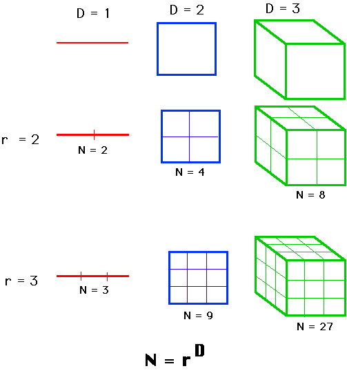 We take the log of both sides, to get
log(N) = D log(r).
Then solve for D.
D = log(N)/log(r)
Examined this way, D need not be an integer. It could be a fraction.
The length of a coastline
Estimate the length by using a rule of length one.
Then halve the ruler, and estimate anew.
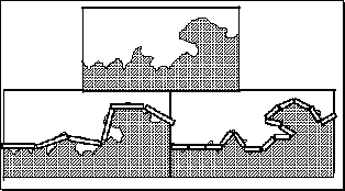 Measuring the length of a coastline using rulers of varying
lengths.
We find that as the ruler decreases, the length continues to increase;
as the ruler gets diminishingly small, the length gets infinitely large.
The concept of length, when applied to the coastline, begins to
make little sense.
The "Richardson Effect"
The relation between length estimate and length of scale is linear
on a log-log plot.
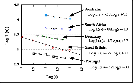 The Richardson Effect.
Mandelbrot assigned the term (1-D) to the slope, so the functions are:
log[L(s)] = (1-D)log(s) + b
where D is the Fractal Dimension.
Examples of geometric objects with non-integer dimensions
Koch Curve
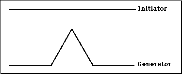 The Initiator and Generator for constructing the Koch
Curve.
 Level 2 in the construction of the Koch Curve.
 Level 3 in the construction of the Koch Curve.
 The Koch Curve.
 What is the length of the Koch curve?
If we treat the Koch curve as we did the coastline, we find its
Fractal dimension to be 1.26. Same result obtained from
D = log(N)/log(r)
D = log(4)/log(3) = 1.26
(More than 1, less than 2).
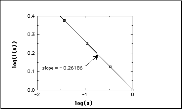 The relation between log(L(s)) and log(s) for the Koch
curve
Cantor Dust
 Initiator and Generator for constructing Cantor Dust.
 Levels 2, 3, and 4 in the construction of Cantor Dust.
D = log(N)/log(r)
D = log(2)/log(3) = .63
An object with dimensionality less than one.
Sierpinski Triangle
We start with an equilateral triangle, connect the mid-points of the three
sides and
remove the resulting inner triangle.
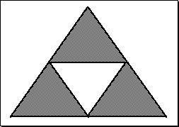 Constructing the Sierpinski Triangle.
Iterating the first step.
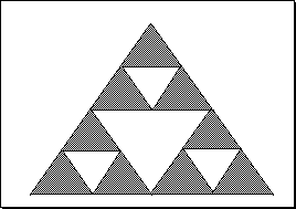 Constructing the Sierpinski Triangle.
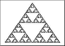 The Sierpinski Triangle.
D = log(N)/log(r) = log(3)/log(2) = 1.585.
The dimensionality of a strange attractor
- The trajectory of a strange attractor cannot interect cross itself. (Why?)
- Nearby trajectories diverge exponentially. (Why?)
- But the attractor is bounded to the phase space.
- The trajectory does not fill the phase space.
It is a fractal, and its fractal dimension is less than the dimensions of its
phase space.
Mandelbrot Set
Found by iterating
z(n+1) = z(n)^2 + c.
where z is a complex number. z(0)=0.
For different values of c, the trajectories either: stay near the origin, or
"escape".
The Mandelbrot set is the set of points that are not in the Escape Set.
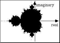 The Mandelbrot set. The points in the set are painted black.
The Escape Set differs in rate of escape, graphically depicted with different
colors or altitudes ...
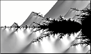 Constructed using the computer program "The Beauty of Fractal
Lab", by
Thomas Eberhardt.

So, what is a fractal?
An irregular geometric object with an infinite nesting of
structure at all scales.
Why do we care about fractals?
- Natural objects are fractals.
- Chaotic trajectories are fractals.
Back to Table of Contents
Return Maps
What is a return map?
A plot of x(t) against x(delta t)
Why is it plotted?
To evaluate the structure of the measured trajectory.
To illustrate, we start with random time series.
Data generated by randomly sampling from (0,1) interval.
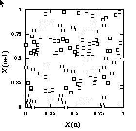 Return Map of time series from random Uniform distribution.
As expected, the points scatter.
Here's a return map from another random time series.
This one sampled from an exponential (positively skewed) distribution.
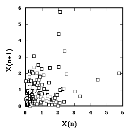 Return Map of time series from exponential distribution.
Here we do not scatter all over, but the axes are still uncorrelated.
Remember this time series?
 A nonrandom Time Series
It's from the Logistic Map in the chaotic region, r=3.99.
What does its Return Map look like?
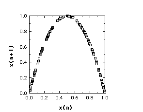 Return Map from Logistic Map, r=3.99
The structure of the generating function is entirely captured.
Embedding dimension
One more meaning of the term 'dimension'.
Comes from operating on a time series.
Successive n- tuples of data are treated as points in n-space.
The Return Map is an embedding dimension of 2.
Suppose, for example, that the first six data values were
4, 2, 6, 1, 5, 3,
then for an embedding dimension of 3.
P(1)= (4,2,6)
P(2)= (2,6,1)
P(3)= (6,1,5), and so forth.
What's the point?
Contemporary statistical analyses examine the geometric structure of obtained time series embedded with differing dimensions.
Nonlinear Dynamics, Psychology, & Life Sciences
So... what have we learned, and what has it to do with our enterprise?
Back to Table of Contents
Abraham, F., Abraham, R., & Shaw, C. D. (1990). A visual introduction to
dynamical systems theory for psychology. Santa Cruz, CA: Aerial Press, Inc.
Lorenz, E. N. (1963). Deterministic non-periodic flows. Journal of
Atmospheric Science, 20, 130-141.
Mandelbrot, B. (1982). The Fractal Geometry of Nature. New York, NY: W. H.
Freeman.
van Geert, P. (1991). A dynamic systems model of cognitive and language
growth. Psychological Review, 98, 3-53.
Back to Table of Contents
Return to Chaos Society